Storing and Accessing Data in Parallelism Friendly Formats
Overview
Teaching: 50 min
Exercises: 30 minQuestions
How can we use an object store to store data that is accessible over the internet?
How do we access data in an object store using Xarray?
Objectives
Understand the relative performance of memory, local disks, local networks and the internet.
Understand that object stores are a convienient and scalable way to store data to be accessed over the internet.
Understand how Zarr files can be structured in an object store friendly way.
Apply Xarray to access Zarr files stored in an object store.
Parallel Filesystems
On many high performance computing (HPC) systems it is common for there to be a large parallel filesystem. These will spread data across a large number of physical disks and servers, when a user requests some data it might be supplied by several servers simultaneously. Since each disk can only supply data so fast (usually between 10s and 100s of megabytes per second) we can achieve faster data access by requesting from several disks spread across several servers. Many parallel filesystems will be configured to provide access speeds of multiple gigabytes per second. However HPC systems also tend to be shared systems with many users all running different tasks at any given time, so the activities of other users will also impact how quickly we can access data.
Object Stores
Object stores are a scalable way to store data in a manner that is readily accessible over the internet. They use the Hyper Text Transfer Protocol (HTTP) or its secure alternatie (HTTPS) to access “objects”. In this case each object will have a unique URL and the appearance of a file on a filesystem. Where object stores differ from traditional filesystem is that there isn’t any directory hierarchy to the objects, although sometimes object stores are configured to give the illusion of this. For example we might create object names that contain path separators. The underlying storage can “stripe” the data of an object across several disks and/or servers to achieve higher throughput speeds in a similar way to the parallel filesystems described above, this can allow object stores to scale very well to store both large numbers of objects and very large individual objects. Some object stores will also replicate an object across several locations to both improve reslience and performance.
Another benefit of object stores is that they allow clients to request just part of an object, this has spawned a number of “cloud optimised” file formats where some metadata describes what can be found in what part of the object and the client then requests only what it needs. This could be especially useful if say we have a very high resolution geospatial dataset and only wish to retreive the part relating to a specific area or we have a dataset which spans a long time period and we’re only interested in a short time period.
One of the most popular object stores is Amazon’s S3 which is used by many websites to store their contents. S3 is accessed via HTTP, typically using the GET method to request and object or using the PUT or DELETE methods. S3 also has a lot of features to manage who can access an object and whether they can only read it or read and write it. Many other object stores copy the S3 protocol both for accessing objects, managing permissions and metadata associated with them.
Zarr files
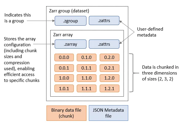
Zarr is a cloud optimised file format designed for working with multidimensional data. Its is very similar to NetCDF, but it splits up data into chunks. When requesting the Zarr file from an object store (or a local disk) we can limit which chunks we transfer. Zarr files contain a header which describes the structure of the file and information about the chunks, when loading the file this header will be loaded to allow the Zarr library to know about the rest of the file. Zarr is also designed to support multiple concurrent readers, allowing us to read the file in parallel using multiple threads or even with Dask tasks that are distributed across multiple computers. Zarr has been built with Python in mind and has libraries to allow native Python operations on Zarr. There is support for Zarr in other languages such as C in the recent versions of the NetCDF libraries.
Zarr and Xarray
Xarray can open Zarr files using the open_zarr function that is similar to the open_dataset function we’ve been using to open NetCDF data.
We will use datasets from dynamical.org, which provides a public, live-updating catalog of weather data in Zarr format. These datasets are stored in an object store and can be several terabytes in size. DO NOT DOWNLOAD THEM LOCALLY.
For example, we can open the ECMWF AIFS model forecast dataset with the following code:
import xarray as xr

ds = xr.open_zarr("https://data.dynamical.org/ecmwf/aifs-single/forecast/latest.zarr")
ds
This dataset includes:
- 3002 initialisation times (
init_time) - 61 lead times (
lead_time) - 721 latitude points
- 1440 longitude points
It contains variables such as:
temperature_2m: temperature at 2 meters above the surfacedew_point_temperature_2m: dew point temperature at 2 meters above the surfacewind_u_10m: zonal wind at 10 meters above the surface
Each variable includes metadata such as units and descriptions. All of this information has come from the header of the Zarr file, so far none of the actual data has been transferred, we have done what is known as a “lazy load” where data will only be transferred from the object store when we actually access it.
In this lesson, we will work with this dataset. You can later explore others in the dynamical.org catalog.
If we inspect temperature_2m, we see that it represents hundreds of gigabytes of data:
ds['temperature_2m']
Let’s try and read it by slicing out a small part of the file. We will slice out the last initialisation time, and get all the lead_times and latitude and longitudes related to it:
temperature_2m = ds['temperature_2m'].isel(init_time=slice(-1, None))
temperature_2m
Now:
init_timeis reduced to 1- the selected time corresponds to the most recent model run (yesterday or today depending on the time of day)
This subset is much smaller, but no data has been loaded yet. If we explore further and print the temperature_2m array we’ll see that it is actually using a Dask array underneath.
print(temperature_2m)
To convert this into a standard Xarray DataArray we can call .compute on the temperature_2m.
temperature_2m_local = temperature_2m.compute()
We can now plot this by selecting the data for the first lead time and then plotting it (we also need to select the first initialisation time since we only have one):
temperature_2m_local.isel(init_time=0, lead_time=0).plot()
Or access some of the data:
temperature_2m_local[0,0,0,0]
If you want to slice the data by the latitude and longitude coordinates you can use sel instead of isel:
temperature_2m_slice = ds['temperature_2m'].sel(latitude=slice(50, 60), longitude=slice(-10, 0))
temperature_2m_slice
Plot the zonal wind at 10 meters above the surface
Extract and plot the sea zonal wind at 10 meters above the surface (
wind_u_10m) variable from the same zarr datasethttps://data.dynamical.org/ecmwf/aifs-single/forecast/latest.zarr) for the initialisation time nearest to January 1st 2025.Solution 1
import xarray as xr
ds = xr.open_zarr("https://data.dynamical.org/ecmwf/aifs-single/forecast/latest.zarr")
wind_u_10m = ds['wind_u_10m'].sel(init_time="2025-01-01",method="nearest")
# note that you already removed the init_time dimension by selecting a single value, so you only need to select the lead_time dimension for plotting
wind_u_10m.isel(lead_time=0).plot()
Solution 2: (OPTIONAL) plotting with Cartopy
import xarray as xr
import matplotlib.pyplot as plt
import cartopy.crs as ccrs
import cartopy.feature as cfeature
ds = xr.open_zarr("https://data.dynamical.org/ecmwf/aifs-single/forecast/latest.zarr")
wind_u_10m = ds['wind_u_10m'].sel(init_time="2025-01-01",method="nearest").isel(lead_time=0)

plt.figure(figsize=(12, 6))
ax = plt.axes(projection=ccrs.PlateCarree())

# Add white land background
ax.add_feature(cfeature.LAND, facecolor='white', zorder=1)

ax.coastlines()
pcm = ax.pcolormesh(
    wind_u_10m.longitude, wind_u_10m.latitude, wind_u_10m,
    transform=ccrs.PlateCarree(),
    cmap="viridis",
    shading="auto",
    zorder=0  # Ensure it overlays the land
)

plt.title("Sea Zonal Wind at 10 Meters Above the Surface")
plt.colorbar(pcm, label=wind_u_10m.attrs.get("units", ""))
plt.tight_layout()
plt.show()
Calculate the mean initialisation temperature for 2 meters above the surface for 15 days
Using the Zarr dataset
https://data.dynamical.org/ecmwf/aifs-single/forecast/latest.zarr, calculate the daily mean initialisation temperature at 2 meters above the surface (temperature_2m) for the first 15 days of January 2025 using Xarray.The initialisation temperature refers to the temperature at the time the model is initialised. To compute this:
- Select the relevant
init_timerange covering the first 15 days of January 2025- Select the first
lead_time(i.e. the time corresponding to the model initialisation)- Compute the mean temperature across the
latitudeandlongitudedimensionsFinally, try increasing the number of days (e.g. to 30 days) and observe how this affects the computation time.
Solution
import xarray as xr
ds = xr.open_zarr("https://data.dynamical.org/ecmwf/aifs-single/forecast/latest.zarr")
temperature_2m = ds['temperature_2m'].sel(
    init_time=slice("2025-01-01", "2025-01-15"),
).isel(lead_time=0)
grouped_mean = temperature_2m.groupby("init_time.day").mean()
mean_temperature_2m = grouped_mean.mean(dim=['latitude','longitude']) # this will take the mean across the specified dimensions
mean_temperature_2m = mean_temperature_2m.compute()
mean_temperature_2m.plot()
print(mean_temperature_2m)
Calculate the initialisation temperature for 2 meters using Dask
Using the Zarr dataset
https://data.dynamical.org/ecmwf/aifs-single/forecast/latest.zarr, calculate the daily mean initialisation temperature at 2 meters above the surface (temperature_2m) for December 2024. Use the JASMIN Dask Gateway to parallelise the computation, with a maximum of 10 worker threads. To complete this task:
- Select the
init_timerange covering all of December 2024- Select the first
lead_time(representing the model initialisation time)- Compute the daily mean temperature across the
latitudeandlongitudedimensions Measure how long the computation takes. Then experiment by increasing and decreasing the number of workers to identify an efficient configuration. You can monitor whether the requested workers are being created on JASMIN using:watch squeue -q dask -u <your user id>Solution
import xarray as xr
import dask_gateway

gw = dask_gateway.Gateway("https://dask-gateway.jasmin.ac.uk", auth="jupyterhub")

options = gw.cluster_options()
options.worker_cores = 1
options.scheduler_cores = 1
options.account = "workshop"
options.worker_setup='source /apps/jasmin/jaspy/miniforge_envs/jaspy3.11/mf3-23.11.0-0/bin/activate /work/scratch-nopw2/colinsau/esces-env'

clusters = gw.list_clusters()
if not clusters:
    cluster = gw.new_cluster(options, shutdown_on_close=False)
else:
    cluster = gw.connect(clusters[0].name)

client = cluster.get_client()
cluster.adapt(minimum=1, maximum=15)
client

ds = xr.open_zarr("https://data.dynamical.org/ecmwf/aifs-single/forecast/latest.zarr")
temperature_2m = ds['temperature_2m'].sel(
    init_time=slice("2024-12-01", "2024-12-31"),
).isel(lead_time=0)
grouped_mean = temperature_2m.groupby("init_time.day").mean()
mean_temperature_2m = grouped_mean.mean(dim=['latitude','longitude'])
result = client.compute(mean_temperature_2m).result()
result.plot()
cluster.shutdown()
Data Catalogues
It is a common problem that environmental scientists will need to work with datasets that span across many files. There is a common practice with larger datasets stored in Zarr or NetCDF formats to split them into multiple files with either one variable per file or one time period per file. Once we have more than a few files in our dataset keeping the correct filenames or URLs can become more difficult, especially if those names change or data gets relocated.
There are several ways to solve this problem, most of then related on building a catalogue of the dataset. This catalogue can be a simple text file that lists the filenames and URLs of the files in the dataset (like this example), or it can be a more complex database or catalogue that stores metadata about the files and their contents.
Two most used catalogues for this type of data are STAC and Intake. STAC is a standard for describing geospatial data in a way that allows it to be easily discovered and accessed, while Intake is a Python library that provides a way to manage and access datasets in a more flexible way. We will show an example using intake.
To open a catalogue we call the open_catalog function in the intake library. By converting the response of this to a Python list we can find the names of all of the datasets
in the catalogue.
import intake
xcat = intake.open_catalog('https://raw.githubusercontent.com/intake/intake-xarray/master/examples/catalog.yml')
list(xcat)
Let’s open the image example and use the skimage library to plot it
import matplotlib.pyplot as plt
image = xcat.image.read()
plt.imshow(image)
Key Points
We can process faster in parallel if we can read or write data in parallel too
Data storage is many times slower than accessing our computer’s memory
Object stores are one way to store data that is accessible over the web/http, allows replication of data and can scale to very large quantities of data.
Zarr is an object store friendly file format intended for storing large array data.
Zarr files are stored in chunks and software such as Xarray can just read the chunks that it needs instead of the whole file.
Xarray can be used to read in Zarr files